

Bar charts are an excellent way to visually represent data comparisons, and Google Sheets offers intuitive tools to create and customize them. Whether you're looking to create a bar graph in Google Sheets or explore options like grouped and stacked bar charts, this guide will walk you through the steps. With features that allow easy customization, Google Sheets bar graph examples can help you present your data clearly and effectively.
1. Bar Graphs
A bar graph is a simple chart that uses bars to show and compare amounts or values across different categories. The length or height of each bar represents the value of that category, making it easy to see differences at a glance.
Key features of bar graphs:
- Categories and Values: The horizontal axis (x-axis) usually shows categories, and the vertical axis (y-axis) shows values.
- Bars: Each bar represents a category, and its size matches the value.
- Clear Spacing: Bars are spaced apart to make each category stand out.
Bar graphs are great for comparing data, like showing sales by month, survey results, or student scores. They are easy to create and understand, making them useful for both simple and complex data comparisons.
2. How to Add Bar Charts in Google Sheets
Here are the easy steps to add and edit Bar charts in Google sheets:
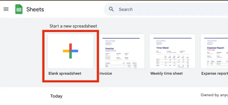
Step 1: Open Google Sheets
Before creating a chart, ensure your data is well-organized. Open Google Sheets and either create a new sheet or use an existing one.
Step 2: Prepare Your Data in Google Sheets
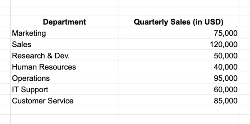
Ensure your data is organized for effective chart creation. Open a new or existing Google Sheets file. Add clear headers for both columns and Organize your data in a table format:
- Place categories (e.g., items, departments) in the first column.
- Place corresponding values (e.g., sales, counts) in the second column.
Step 3: Highlight Your Data
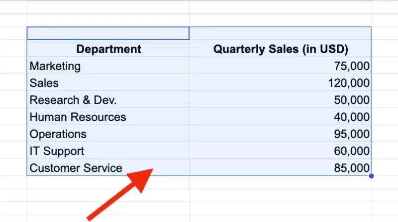
Use your cursor to highlight the data range, including headers, that you want in the bar chart.
Example: Highlight cells A1 to B10.
Step 4: Insert the Chart
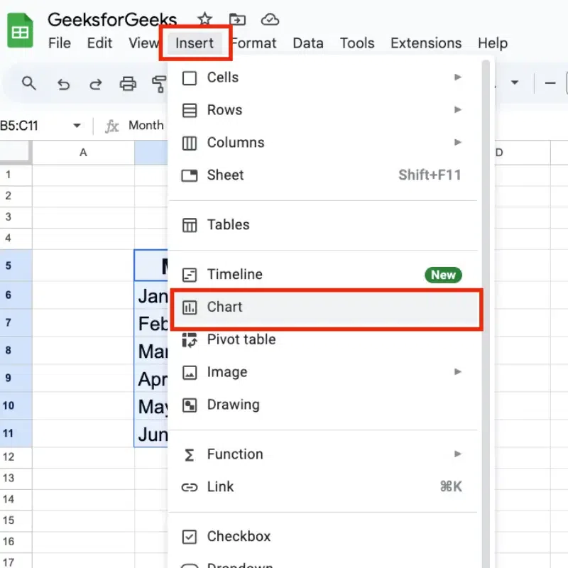
Go to the Insert menu in the top toolbar. Select Chart from the dropdown menu.
Step 5: See the Chart
A default chart will appear in your sheet.
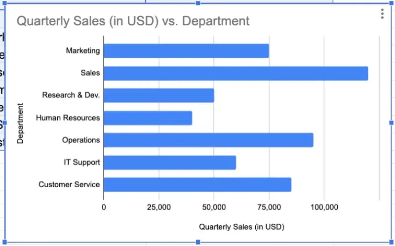
Step 5: Change the Chart Type to Bar Chart
- Open the Chart Editor panel on the right.
- Under the Setup tab, locate the Chart type dropdown menu.
- Scroll and select Bar chart (not column chart). The chart will update accordingly.
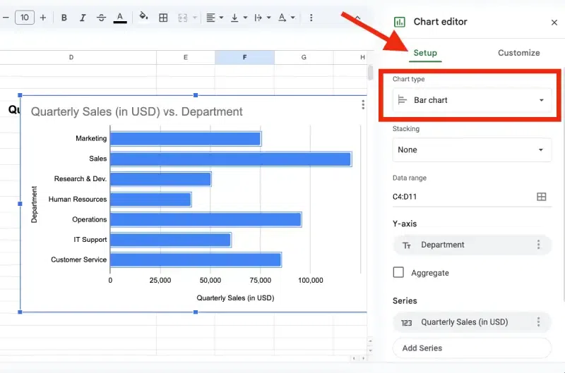
Step 6: Customize the Bar Chart
Fine-tune your chart to make it visually clear and informative. Go to the Customize tab in the Chart Editor. Adjust these key settings:
- Chart Title: Add a descriptive title under Chart & axis titles.
- Colors: Change bar colors under Series to differentiate data categories.
- Gridlines and Ticks: Add or remove gridlines for better clarity.
- Horizontal vs. Vertical Bars: Ensure the data orientation matches your presentation needs.

Step 7: Resize and Reposition the Chart
- Click on the chart to select it.
- Drag the chart to the desired position on your sheet.
- Adjust the size by dragging the corners of the chart.
Step 8: Save and Share the Chart
To download the chart, Right-click on the chart and choose Save image. Alternatively, copy and paste the chart into another document or presentation.
To share the chart:
- Click Share in the top-right corner of Google Sheets.
- Set sharing permissions and send the link to collaborators.
3. Types of Bar Charts in Google Sheets
Google Sheets supports several bar chart variations for different insights.
1. Horizontal Bar Chart
Bars run horizontally; ideal for long category names.
Steps
- Follow basic insertion.
- In Chart editor > Setup > Chart type, select Bar chart (horizontal by default for category-heavy data).
Use Case: Comparing department budgets with lengthy names.
2. Stacked Bar Chart
Stacks segments within bars to show parts of a whole.
Steps
- Select multi-series data (e.g., A1:D6).
- Insert chart.
- In Chart editor > Setup > Chart type, select Stacked bar chart.
Use Case: Visualizing quarterly sales contributions by region (total bar = overall sales).
3. Grouped Bar Chart
Groups bars side-by-side for multi-series comparisons.
Steps
- Select data.
- Insert chart.
- In Chart editor > Setup > Chart type, select Bar chart (default for multi-series is grouped).
Use Case: Comparing Q1, Q2, Q3 sales across regions.
Tip: Switch between stacked/grouped in Setup > Stacking.
