


VICReg: Variance-Invariance-Covariance Regularization for Self-Supervised Learning
VICReg:用于自监督学习的方差-不变性-协方差正则化
【2021-05】VICReg:方差-不变性-协方差正则化的自监督联合嵌入学习【同图双视图编码对齐;批次中每行对应一张图、每列对应一个特征维度;列内方差防止表示坍塌,列间协方差抑制特征冗余,无负样本】
Abstract
摘要
Recent self-supervised methods for image representation learning maximize the agreement between embedding vectors produced by encoders fed with different views of the same image. The main challenge is to prevent a collapse in which the encoders produce constant or non-informative vectors. We introduce VICReg (Variance-Invariance-Covariance Regularization), a method that explicitly avoids the collapse problem with two regularizations terms applied to both embeddings separately:
- (1) a term that maintains the variance of each embedding dimension above a threshold,
- (2) a term that decorrelates each pair of variables.
Unlike most other approaches to the same problem, VICReg does not require techniques such as: weight sharing between the branches, batch normalization, feature-wise normalization, output quantization, stop gradient, memory banks, etc., and achieves results on par with the state of the art on several downstream tasks. In addition, we show that our variance regularization term stabilizes the training of other methods and leads to performance improvements.
最近的图像表征学习自监督方法通过最大化由输入同一图像不同视图的编码器生成的Embedding 向量之间的一致性来进行学习。
主要挑战是防止发生坍塌,即编码器生成恒定或无信息的向量。
我们提出了VICReg (Variance-Invariance-Covariance Regularization),—种通过分别应用于两个Embedding的两项正则化来显式避免坍塌问题的方法:
- (1)使每个Embedding 维度的方差保持在阈值以上的项;
- (2)对每一对变量进行去相关的项。
与大多数解决相同问题的其他方法不同,VICReg不需要诸如以下技术:
- 分支之间的权重共享、
- 批归一化、
- 按特征归一化、
- 输出Quantization、
- 停止梯度、
- 记忆库等,
并且在多项下游任务上取得了与最先进方法相当的结果。
此外,我们表明,方差正则化项能够稳定其他方法的训练,并带来性能提升。
1引言
Self-supervised representation learning has made significant progress over the last years, almost reaching the performance of supervised baselines on many downstream tasks Bachman et al. (2019); Misra & Maaten (2020); He et al. (2020); Tian et al. (2020); Caron et al. (2020); Grill et al. (2020); Chen & He (2020); Gidaris et al. (2021); Zbontar et al. (2021). Several recent approaches rely on a joint embedding architecture in which two networks are trained to produce similar embeddings for different views of the same image. A popular instance is the Siamese network architecture Bromley et al. (1994), where the two networks share the same weights. The main challenge with joint embedding architectures is to prevent a collapse in which the two branches ignore the inputs and produce identical and constant output vectors. There are two main approaches to preventing collapse: contrastive methods and information maximization methods. Contrastive Bromley et al. (1994); Chopra et al. (2005); He et al. (2020); Hjelm et al. (2019); Chen et al. (2020a) methods tend to be costly, require large batch sizes or memory banks, and use a loss that explicitly pushes the embeddings of dissimilar images away from each other. They often require a mining procedure to search for offending dissimilar samples from a memory bank He et al. (2020) or from the current batch Chen et al. (2020a). Quantization-based approaches Caron et al. (2020; 2018) force the embeddings of different samples to belong to different clusters on the unit sphere. Collapse is prevented by ensuring that the assignment of samples to clusters is as uniform as possible. A similarity term encourages the cluster assignment score vectors from the two branches to be similar. More recently, a few methods have appeared that do not rely on contrastive samples or vector quantization, yet produce high-quality representations, for example BYOL Grill et al. (2o2o) and SimSiam Chen & He (2o2o). They exploit several tricks: batch-wise or feature-wise normalization, a “momentum encoder” in which the parameter vector of one branch is a low-pass-filtered version of the parameter vector of the other branch Grill et al. (2020); Richemond et al. (2020), or a stop-gradient operation in one of the branches Chen & He (2020). The dynamics of learning in these methods, and how they avoid collapse, is not fully understood, although theoretical and empirical studies point to the crucial importance of batch-wise or feature-wise normalization Richemond et al. (2o2o); Tian et al. (2021).
自监督表征学习在过去几年中取得了显著进展,在许多下游任务上的性能几乎达到了监督学习基线的水平 Bachman etal. (2019); Misra & Maaten (2020); He et al. (2020); Tian et al. (2020); Caron et al. (2020); Grill et al. (2020);Chen & He (2020); Gidaris et al. (2021); Zbontar et al. (2021)。
—些近期方法依赖于联合 Embedding 架构,其中训练两个网络,使其针对同一图像的不同视图产生相似的 Embedding。
一个常见实例是孪生网络架构 Bromley et al.(1994),其中两个网络共享相同的权重。
联合Embedding 架构面临的主要挑战是防止发生坍塌,即两个分支忽略输入并产生相同且恒定的输出向量。
防止坍塌主要有两种方法:对比方法和信息最大化方法。
- 对比学习方法 Bromley et al.(1994): Chopra et al. (2005): He et al. (2020): Hielm et al. (2019): Chen et al. (2020a) 往往成本较高, 需要较大的批次大小或记忆库,并且使用一种显式地将不相似图像的Embedding相互推远的损失函数。它们通常需要一个挖掘过程,从记忆库 He et al. (2020) 或当前批次 Chen et al. (2020a) 中搜索有问题的不相似样本。
- 基于 Quantization 的方法 Caron et al. (2020; 2018) 强制不同样本的 Embedding 属于单位球面上的不同簇。通过确保样本到簇的分配尽可能均匀来防止坍塌。相似性项鼓励两个分支的簇分配得分向量彼此相似。
最近,出现了一些既不依赖对比样本也不依赖向量 Quantization、但仍能产生高质量表征的方法,例如 BYOL Grill et al.(2020) 和 SimSiam Chen & He(2020)。
它们利用了多种技巧:
- 按批次或按特征进行归一化;“动量编码器”,其中一个分支的Parameter 向量是另一个分支的Parameter 向量的低通滤波版本 Grill et al. (2020); Richemond et al. (2020);
- 或者在其中—个分支中使用停止梯度操作 Chen & He(2020)。
这些方法的学习动态及其如何避免坍塌尚未被完全理解,尽管理论和实证研究都指出,按批次或按特征进行归一化至关重要 Richemond et al. (2020); Tian et al. (2021)。
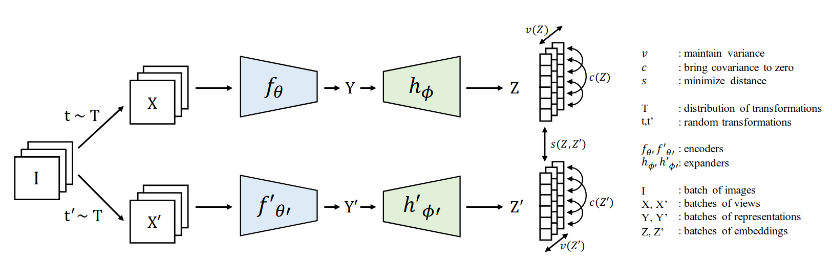
Figure 1: VICReg: joint embedding architecture with variance, invariance and covariance regularization. Given a batch of images III, two batches of different views XXX and X′X'X′ are produced and are then encoded into representations YYY and Y′Y'Y′. The representations are fed to an expander producing the embeddings ZZZ and Z′Z'Z′. The distance between two embeddings from the same image is minimized, the variance of each embedding variable over a batch is maintained above a threshold, and the covariance between pairs of embedding variables over a batch are attracted to zero, decorrelating the variables from each other. Although the two branches do not require identical architectures nor share weights, in most of our experiments, they are Siamese with shared weights: the encoders are ResNet-50 backbones with output dimension 2048. The expanders have 3 fully-connected layers of size 8192.
图 1:VICReg:具有方差、不变性和协方差正则化的联合嵌入架构。
- 给定一批图像 III,
- 生成两批不同的视图 XXX 和 X′X'X′,随后将它们编码为表示 YYY 和 Y′Y'Y′。
- 这些表示被输入到一个扩展器中,从而产生嵌入 ZZZ 和 Z′Z'Z′。
- 来自同一图像的两个嵌入之间的距离被最小化;
- 每个嵌入变量在一个批次上的方差被维持在某个阈值以上;
- 同时,一个批次上各对嵌入变量之间的协方差被拉向零,从而使这些变量彼此去相关。
- 尽管两个分支不要求具有相同的架构,也不要求共享权重,但在我们的大多数实验中,它们采用共享权重的孪生结构:编码器是输出维度为 2048 的 ResNet-50 主干网络。扩展器包含 3 个大小为 8192 的全连接层。
Finally, an alternative class of collapse prevention methods relies on maximizing the information content of the embedding Zbontar et al. (2021); Ermolov et al. (2021). These methods prevent informational collapse by decorrelating every pair of variables of the embedding vectors. This indirectly maximizes the information content of the embedding vectors. The Barlow Twins method drives the normalized cross-correlation matrix of the two embeddings towards the identity Zbontar et al. (2o21), while the Whitening-MSE method whitens and spreads out the embedding vectors on the unit sphere Ermolov et al. (2o21).
最后,一个另一类防止塌缩的方法依赖于最大化 Embedding 的信息内容 Zbontar et al. (2021); Ermolov et al.(2021)。这些方法通过去除Embedding 向量中每一对变量之间的相关性来防止信息塌缩。这间接最大化了Embedding 向量的信息内容。Barlow Twins 方法将两个 Embedding 的归一化互相关矩阵推向单位矩阵 Zbontar et al.(2021),而 Whitening-MSE 方法对白化 Embedding 向量,并将其分散在单位球面上 Ermolov et al. (2021)。
2 VICReg: INTUITION
2 VICReg:直觉
We introduce VICReg (Variance-Invariance-Covariance Regularization), a self-supervised method for training joint embedding architectures based on the principle of preserving the information content of the embeddings. The basic idea is to use a loss function with three terms:
我们提出了 VICReg(方差-不变性-协方差正则化),这是一种用于训练联合Embedding 架构的自监督方法,其基于保持 Embedding 信息内容的原则。其基本思想是使用一个包含三项的 Loss Function:
-
Invariance: the mean square distance between the embedding vectors.
-
不变性:Embedding 向量之间的均方距离。
-
Variance: a hinge loss to maintain the standard deviation (over a batch) of each variable of the embedding above a given threshold. This term forces the embedding vectors of samples within a batch to be different.
-
方差:一种铰链损失,用于将Embedding 中每个变量的标准差(在一个批次内)保持在给定阈值之上。该项迫使一个批次内样本的 Embedding 向量彼此不同。
-
Covariance: a term that attracts the covariances (over a batch) between every pair of (centered) embedding variables towards zero. This term decorrelates the variables of each embedding and prevents an informational collapse in which the variables would vary together or be highly correlated.
-
协方差:一种使每对(中心化)Embedding变量之间的协方差(在一个批次内)趋近于零的项。该项对每个Embedding的变量进行去相关处理,并防止信息坍塌,即变量会共同变化或高度相关。
可以把这句话概括为:
VICReg 通过三个损失共同训练网络:让同一图片的不同增强表示接近,同时保证不同图片的表示不会全部坍塌,并让不同嵌入维度尽量减少线性重复。
其中,方差正则化与协方差正则化最终希望网络输出的协方差矩阵呈现:
C(Z)≈diag(s12,s22,…,sD2),sj≥γC(Z)\approx\operatorname{diag}(s_1^2,s_2^2,\ldots,s_D^2),\qquad s_j\geq\gammaC(Z)≈diag(s12,s22,…,sD2),sj≥γ
也就是:
- 对角元素不能太小:每个特征维度必须有足够变化;
- 非对角元素尽量接近 0:不同特征维度尽量线性去相关。
2.1、5 张图片如何形成嵌入矩阵
假设一个 batch 中有 5 张不同的原始图片:
x1,x2,x3,x4,x5x_1,x_2,x_3,x_4,x_5x1,x2,x3,x4,x5
每张图片生成两个随机增强视图:
xi(1)=ti(1)(xi),xi(2)=ti(2)(xi)x_i^{(1)}=t_i^{(1)}(x_i),\qquad x_i^{(2)}=t_i^{(2)}(x_i)xi(1)=ti(1)(xi),xi(2)=ti(2)(xi)
两个分支分别得到嵌入矩阵:
Z=fθ(X(1)),Z′=fθ(X(2))Z=f_\theta(X^{(1)}),\qquad Z'=f_\theta(X^{(2)})Z=fθ(X(1)),Z′=fθ(X(2))
其中:
Z,Z′∈R5×DZ,Z'\in\mathbb R^{5\times D}Z,Z′∈R5×D
为方便展示,假设嵌入维度为 D=3D=3D=3:
Z=[z11z12z13z21z22z23z31z32z33z41z42z43z51z52z53]Z=\begin{bmatrix}z_{11}&z_{12}&z_{13}\\z_{21}&z_{22}&z_{23}\\z_{31}&z_{32}&z_{33}\\z_{41}&z_{42}&z_{43}\\z_{51}&z_{52}&z_{53}\end{bmatrix}Z= z11z21z31z41z51z12z22z32z42z52z13z23z33z43z53
这里:
- 每一行表示一张图片的完整嵌入;
- 每一列表示同一个嵌入变量在 5 张图片上的输出。
例如第一列:
Z:,1=[z11,z21,z31,z41,z51]⊤Z_{:,1}=[z_{11},z_{21},z_{31},z_{41},z_{51}]^\topZ:,1=[z11,z21,z31,z41,z51]⊤
表示第一个特征维度对 5 张不同图片的响应。
2.2、这里的“正则化”是什么意思
正则化是指:
在主要学习目标之外加入额外约束,排除不合理或退化的解,引导模型学习更有用的表示。
VICReg 的总损失可以写成:
L=λLinv+μLvar+νLcov\mathcal L=\lambda\mathcal L_{\mathrm{inv}}+\mu\mathcal L_{\mathrm{var}}+\nu\mathcal L_{\mathrm{cov}}L=λLinv+μLvar+νLcov
其中:
| 损失 | 约束 |
|---|---|
| Linv\mathcal L_{\mathrm{inv}}Linv | 同一图片的两个增强表示应当接近 |
| Lvar\mathcal L_{\mathrm{var}}Lvar | 每个嵌入维度在不同图片之间要有足够变化 |
| Lcov\mathcal L_{\mathrm{cov}}Lcov | 不同嵌入维度不要重复同一种线性变化模式 |
这里的正则化不是简单地“把数值变小”。
- 方差正则化反而防止标准差太小;
- 协方差正则化才要求非对角协方差变小。
2.3、不变性损失:同一图片的两个视图靠近
第 iii 张原始图片的两个增强视图分别得到:
zi,zi′\mathbf z_i,\qquad\mathbf z_i'zi,zi′
不变性损失通常采用均方误差:
Linv(Z,Z′)=15∑i=15∥zi−zi′∥22\mathcal L_{\mathrm{inv}}(Z,Z')=\frac{1}{5}\sum_{i=1}^{5}\|\mathbf z_i-\mathbf z_i'\|_2^2Linv(Z,Z′)=51i=1∑5∥zi−zi′∥22
它要求:
zi≈zi′\mathbf z_i\approx\mathbf z_i'zi≈zi′
也就是同一张图片经过裁剪、翻转、颜色扰动等增强后,语义表示仍应接近。
但是,如果只使用不变性损失,网络可以选择一个无意义的解:
z1=z2=⋯=z5=c\mathbf z_1=\mathbf z_2=\cdots=\mathbf z_5=\mathbf cz1=z2=⋯=z5=c
所有图片都输出同一个向量时,同一图片的两个视图当然完全相同,因此不变性损失可能为 0。
这就是表征坍塌。所以还必须加入方差正则化。
2.4、方差正则化:每一列必须有足够变化
4.1 按列计算标准差
对于第 jjj 个嵌入变量,其 batch 均值是:
μj=15∑i=15zij\mu_j=\frac{1}{5}\sum_{i=1}^{5}z_{ij}μj=51i=1∑5zij
样本方差是:
sj2=14∑i=15(zij−μj)2s_j^2=\frac{1}{4}\sum_{i=1}^{5}(z_{ij}-\mu_j)^2sj2=41i=1∑5(zij−μj)2
标准差是:
sj=14∑i=15(zij−μj)2+ϵs_j=\sqrt{\frac{1}{4}\sum_{i=1}^{5}(z_{ij}-\mu_j)^2+\epsilon}sj=41i=1∑5(zij−μj)2+ϵ
这里分母是 5−1=45-1=45−1=4,ϵ\epsilonϵ 是用于数值稳定的小正数。
VICReg 的单分支方差损失为:
Lvar(Z)=1D∑j=1Dmax(0,γ−sj)\mathcal L_{\mathrm{var}}(Z)=\frac{1}{D}\sum_{j=1}^{D}\max(0,\gamma-s_j)Lvar(Z)=D1j=1∑Dmax(0,γ−sj)
完整的双分支形式通常为:
Lvar=Lvar(Z)+Lvar(Z′)\mathcal L_{\mathrm{var}}=\mathcal L_{\mathrm{var}}(Z)+\mathcal L_{\mathrm{var}}(Z')Lvar=Lvar(Z)+Lvar(Z′)
有些实现会再除以 2,这只改变整体缩放。
2.4.2 阈值 γ\gammaγ 的意义
通常取:
γ=1\gamma=1γ=1
对于某个维度:
| 标准差 sjs_jsj | 该维度的方差惩罚 |
|---|---|
| 000 | 111 |
| 0.40.40.4 | 0.60.60.6 |
| 0.90.90.9 | 0.10.10.1 |
| 111 | 000 |
| 1.51.51.5 | 000 |
因此,方差正则化不是要求标准差无限变大,而只是要求:
sj≥γs_j\geq\gammasj≥γ
一旦达到阈值,就不再继续放大这一维。
2.4.3 为什么按列正则化
假设某一列为:
Z:,1=[0.5,0.5,0.5,0.5,0.5]⊤Z_{:,1}=[0.5,0.5,0.5,0.5,0.5]^\topZ:,1=[0.5,0.5,0.5,0.5,0.5]⊤
那么:
s1=0s_1=0s1=0
这意味着无论输入哪张图片,第一个特征维度都输出 0.50.50.5。该维度完全没有区分能力。
如果所有列都如此,则:
z1=z2=⋯=z5\mathbf z_1=\mathbf z_2=\cdots=\mathbf z_5z1=z2=⋯=z5
网络无法区分这 5 张图片。
因此,方差正则化的核心作用是:
保证每个嵌入维度都对不同图片产生足够不同的响应,防止维度退化为常数,进而防止整体表征坍塌。
2.5、协方差正则化:不同列不要重复变化
方差正则化只能保证“每一列都有变化”,但不能保证“不同列携带不同信息”。
例如:
Z:,2=Z:,1Z_{:,2}=Z_{:,1}Z:,2=Z:,1
第一列和第二列虽然都有较大方差,但第二列只是第一列的复制品。
2.5.1 先对每一列中心化
定义中心化矩阵:
Z~=Z−1μ⊤\widetilde Z=Z-\mathbf1\boldsymbol\mu^\topZ =Z−1μ⊤
其中:
μ=[μ1,μ2,…,μD]⊤\boldsymbol\mu=[\mu_1,\mu_2,\ldots,\mu_D]^\topμ=[μ1,μ2,…,μD]⊤
中心化只是减去每列均值,不是提前去除相关性。
然后计算协方差矩阵:
C(Z)=14Z~⊤Z~C(Z)=\frac{1}{4}\widetilde Z^\top\widetilde ZC(Z)=41Z ⊤Z
对于三维嵌入:
C(Z)=[C11C12C13C21C22C23C31C32C33]C(Z)=\begin{bmatrix}C_{11}&C_{12}&C_{13}\\C_{21}&C_{22}&C_{23}\\C_{31}&C_{32}&C_{33}\end{bmatrix}




 扫一扫
扫一扫


 261
261

 被折叠的 条评论
为什么被折叠?
被折叠的 条评论
为什么被折叠?
 到【灌水乐园】发言


